International Journal of Mining, Materials, and Metallurgical Engineering (IJMMME)

ISSN: 2562-4571

Nomenclature:

• Pressure in the point
• Gravitational constant
• Density in the point
• Friction losses from point  to
• Losses factor as a contribution of pipe section and accessories
• Linear velocity of fluid in
• Pressure drop in a sudden contraction
• Correction factor for in a sudden contraction
• Relation between the diameters in a sudden contraction
• Mass flow in the point
• The Rosin-Rammler function
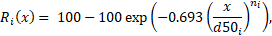
• The cut diameter of solid separation
• The particle size
• Parameter of the Rosin-Rammler function
• The volume fraction of solids
• The mass fraction
• The dry base mass fraction
• The solid concentration
• Number of turns of particles travel by trajectory
• Energy loss due to the travel in a spiral
• Friction Darcy factor
• Curvature radio of the spiral
• Vortex diameter
• Air-core diameter
• Hidrocyclone diameter

1. Introduction

Nowadays, the effort to understand and quantify the separation mechanism in hydrocyclones can be classified from a point of view extremely theoretic or empiric [1]. Although these separation equipments are widely used in the mineral processing industry to classify solids due to high separation efficiency and the relative easy operation, the design and modeling have been majority heuristic. Probably, the reason is due to the complexity of the involved phenomena. For empirical models, Murthy & Bhaskar [2] mentioned that the most used models were developed by Lynch & Rao in 1975 and Plitt in 1976. However, these models can only be applied around the operating point where the experimental data were taken [2], [3]. We want to point out that the empirical models cannot provide the phenomenological knowledge of the system because that kind of models only considers the system as a set of inputs/outputs without taking into account the involved physical principles.

On the other hand, the theoretical models based on first principles have been recently considered to understand the dynamics involved in this kind of separation process. The most relevant approaches correspond to the full and simplified Eulerian multiphase models [4], [5], which are solved using computational fluid dynamics (CFD). However, the high computational effort makes impossible its use in real time operation.

The task of this work is to provide a hydrocyclone model based on physical principles for which the compromise between accuracy and computation effort is considered, allowing its use in real time operation. This model provides an easier approach to simulate the material processing and handling using hydrocyclones. In addition, the model can be used to predict the behavior of a mineral processing plant as a whole. These uses contribute to a plantwide control of such a class of plants known as difficult to optimize regarding their particles separation performance.

The paper is organized as it follows. The so-called Phenomenological-Based Semiphysical Modeling (PBSM) approach [6] is developed in Section 2. In Section 3 the prediction of efficiency of the separation process and the feasible operation region are computed using the simulated model. Conclusions are given in Section 4.

2. Mathematical Model

It is said that a model is phenomenological based when its structure is developed through process matter, energy and momentum balances, and it can be also semiphysical when empirical formulations for various parameters are used as a part of the model [6], [7]. These families of models, specifically using concentrated parameters, have been commonly used in process analysis, design and control. In this sense, and looking for clarifying the model presentation, the ten steps of the procedure to obtain a Phenomenological Based Semi-physical Model (PBSM) is repeated here as follows:

1. Develop a verbal description and a process flow diagram that complement each other. These pieces of information must be clear and complete. Description and diagram are doing reference to the real process to be modeled.
2. Propose a modeling hypothesis and set a level of detail for the model according to model object or purpose. Two main options there exist: lumped parameters or distributed parameters.
3. Define as many process systems (PS) on the process to be modeled as required by the level of detail set. A clue to PS determination is to look for physical walls into the process, distinguishable phases or any mass characteristics marking spatial differences.
4. Apply the principle of conservation on each determined PS. It is recommended to take almost next balances: total mass balance, n component mass balances, total energy balances. Mechanical energy balances are indicated when significant pressure or density changes are presumed. This set of equation are the Dynamics Balance Equation (DBE), considering by default that all balances are originally dynamics but can be turned to static if the process has this behavior.
5. Select from DBE those equations with significant information for fulfill the model porpoise established in step 2. Ever some DBE are redundant or are merely a numerical equality.
6. Identify parameters, variables, and constants of the model. Fixed the values for all constant of the model. Remember that variables values will be found by the model after its solution.
7. Find constitutive equations for calculating the largest number of parameters in each processing system. Parameters without a constitutive equation must be identified from experimental data.
8. Verify the Degree of Freedom (DF) of the model (mathematical systems formed by all equations and constant values). DF=Number of equations - Number of unknown variables or parameters. DF must be zero for a solvable model.
9. Build a computational model: a computer program able to solve the model.
10. Validate the model response using real operating conditions related to those used at step 2 for establish the model objective.

One of the key elements during process model construction is to establish an appropriate modeling hypothesis. When a Phenomenological Based Semi-physical Model (PBSM) is being constructed, some assumptions about the phenomena taken place must be formulated. Those assumptions are normally dedicated to declare as constant some variables of the process. There are a group of considerations sometimes called assumptions too, but very different of fixing variables to given values. To these considerations is better to call as modeling hypothesis. Such a hypothesis is based on one or more abstraction of the current phenomena into pre-stated phenomena, easily linked to but simpler than current process phenomena. This abstraction suggest to create a mental image conformed by enough pre-stated phenomena in order to cover interesting characteristics of the process and to write a description of real process behavior using the abstraction. That description is the modeling hypothesis. In this way, the final representation seems like the real phenomena and gives the opportunity of simulate real behaviors using supposed pre-stated behaviors.

The power of this approach is evident because consolidated knowledge is used for constructing new knowledge, which ends validated for the new phenomena model. Note that abstraction does not try to offer an explanation about the real mechanism of the modeled process. Instead of that, abstraction has the intention of facilitating to the user a fast way to model the process without loss the rigor and formalism. In addition, modular construction will help to model complex processes ever the process can be broken into single parts and each one of those parts can be modeled by pre-stated phenomena. In the next section we state the modeling hypothesis to develop the hydrocyclone model.

2. 1. Modeling Hypothesis

To develop the PBSM for the hydrocyclone, the following assumptions, which are inspired by [3], [8] are considered:

• The pressure loss at the feed nozzle of the hydrocyclone is computed using a modified pressure loss formulation for a venturi, which represents suitably the recovered pressure after the contraction.
• After the nozzle, the feed flow splits in two flows, namely underflow (UF) and overflow (OF). Both flows create hypothetical spiral paths in hypothetical pipe form, which travel together until a point where the overflow changes its direction. Thus, the overflow is characterized according to its direction, namely down overflow and up overflow.
• The up overflow pipe is bounded by the air core and the vortex finder, while the underflow pipe is bounded by the hydrocyclone wall and the down overflow pipe.
• The cross-area of each hypothetical pipe is constant through each path.
• The particles moving through the underflow pipe describe a unique trajectory, i.e., the particles do not have independent movements as considered in other models [8].
 
• The pulp movement uses the available energy by each branch.

According to Pana-Suppamassadu & Amnuaypanich [9] there exists a critical inner pressure for which the number of turns for each spiral and the average velocity of the fluid are maximum. Therefore, we assume that the number of turns for each pipe is not fixed but it depends of the inner pressure, the solid concentration of each stream and the liquid-solid properties.

Due to our model is based on transport of a pulp (solids and water) through spirals of a hypothetical pipe, the cross-area of each pipe must be computed. To this end, the air core plays an important role because it determines the suitable operation of the hydrocyclone and bounds the diameter of the cross-area of the up overflow. The air-core is considered as an invariant, i.e., the diameter does not change once a stable operating point is reached. The air core formation is due to the driven machine (fan) effect of the inner vortexes [10], [11].

2. 2. Mass and Energy Balances

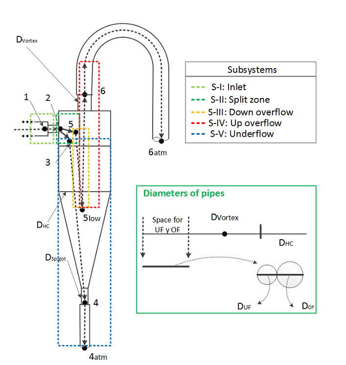
In order to establish the mass and energy balances, we consider the five subsystems sketched in Figure 1.

• S-I: From point 1, inlet of the hydrocyclone, to point 2, the hydrocyclone nozzle input.
• S-II: From point 2, to points 3 and 5. Here we consider the hypothetical split.
• S-III: The down overflow spiral from point 5 to 5low.
• S-IV: The up overflow spiral from point 5low to 6atm.
• S-V: The underflow spiral from point to 4atm.

We assume that the pulp is incompressible and for each subsystem no heat transfer occurs. The drop pressure between points 1 and 2 corresponds to a sudden contraction, which is modeled as a Venturi flowmeter. As assumed above, at point 2 the feed stream splits in two hypothetical pipes, namely, the underflow and overflow. At this split point, the pressures P₂, P₃ and P₅ are assumed to be equal. The particles moving in the overflow pipe descend until a point where a hypothetical pressure P_5low is reached. At this point, the particles change the direction and ascend until the point 6, located at output of the vortex finder. On the other hand, the particles moving in the underflow pipe reach the point 4 which is located in the output of the apex. Between the points 4-4atm and 6-6atm, the losses correspond to the transport in the pipe and the output pressures correspond to the atmospheric pressure. No restrictions at hydrocyclone outputs were assumed but they can be included.

The mechanical energy balance for each subsystem where the pipe section is considered with constant cross-area, gives the following:

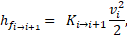
where  is the pressure, g the gravity,  the density,  the height with respect to the hydrocyclone input, and  is the friction loss between points i to i+1. The indexes i and i+1 represent the input and output points in considered hypothetical pipe section.

The friction losses  are computed according to the 2-K method [12],

where,  is the fluid flow linear velocity, and  is a factor computed as a contribution of pipe section and accessories [13].  

For S-I, the hydrocyclone nozzle at the entry is modeled as a venturi flow-meter. Thus, a sudden contraction term,  is consider in Eq. (1),

 is computed from the expression to compute the velocity at venturi throat [11], i.e.,

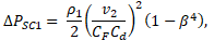
where  is the fluid flow linear velocity,  for Reynolds number between 10.000 and 100.000,  is a correction factor for  by multiphase flow, and  is the relation between the diameter of throat and the diameter of the inlet line.

In S-II we only consider the split into two streams, namely underflow and overflow. Energy losses caused at that point are not considered. In order to characterize the particle size distribution (PSD) for each stream (feed, underflow and overflow), three range of particle sizes (μm) are considered, namely, . The material balance results trivial,

where  represents the mass flow in each stream.

To analyze the particle size distribution in each stream, we first compute the solid volumetric fraction of a given range of particles sizes using the following expression

 

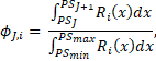
where ,  are the minimum and maximum particle size of fraction J, respectively. ,  are the minimum and maximum particle size in the pulp, respectively.  is the cumulative distribution Rosin-Rammler function,

where  is the cut point of solid separation in the hydrocyclone,  is the particle size, and  is a parameter that must be identified using experiments.  is employed to predict the separation efficiency. Once the volume fractions  are computed, the mass fraction  can be determined using the dry base mass fraction  and the solid concentration ,

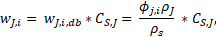
where  is the material density and  is the solid total density. Using the mass fractions , the density  and viscosity  of the pulp can be computed by the following expressions [14],

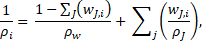
where  is the water density,  the water viscosity, and ,  and  are empirical parameters identified using experiments.

For S-III, IV and V, we apply the Bernoulli's Eq. 1 taking into account that these hypothetical trajectories are spirals with a constant cross-section area. The friction losses for each spiral are computed using Eq. 2, for which the term  is computed as follows

where  is the number of turns that the particles travel in each trajectory and  is the energy loss due to the travel in a spiral. In the proposed model the number of spirals is computed as a function of the inlet pressure  after internal flow splitting, while  is computed using the following equation [15],

where  is the friction Darcy factor,  is the curvature radio of the spiral,  the diameter of the hypothetical pipe and  is a compensation term for a turn in the hypothetical pipe. We want to point out that  is bounded according to the considered subsystem, i.e., for the down overflow (S-III)  is a function of the vortex finder diameter, , and the hypothetical underflow pipe diameter, while for the up overflow (S-IV) the air-core diameter, , reduces the space where this spiral can travel. In spite of a lot of proposals available from literature, the formulation presented in [14] is use as following to compute the air-core diameter,

where is the hidrocyclone diameter,  the nozzle diameter, and the parameters  are identified using experiments.

Thus, the complete model corresponds to the set of equations developed for each subsystem and some constitutive equations related with fluid mechanics which have been avoided for simplicity of the presentation. The resulting model contains 92 nonlinear algebraic equations. As we mention above, some of the model parameters were identified using experiments taken form a pilot plant. The other ones correspond to hydrocyclone geometry and operational parameters. The model was solved in less than 1 second in core-five computer.

3. Results

During parameters identification of the model several assumptions were verified directly on experimental assembly. One of the major facts was the existence of spirals inside the hydrocyclone body. It was evident from direct contact with inside part of hydrocyclone where deep channels were found caused by solids flowing as a part of the pulp. Those channels have a perfect spiral form, indicating that main part of our modeling hypothesis is right. Other verified assumption during experimental section was that of air-core as a physical limit for up overflow inside the hydrocyclone. It was confirmed that when air-core disappears the hydrocyclone operation is totally abnormal.

3. 1. Model Validation

In order to validate the proposed model, several tests were conducted under variation of feed pressure but maintaining feed pulp concentration. At each test three samples were taken during hydrocyclone operation: one of feed pulp, a second from overflow conduction and the third from underflow stream. The model was fed with next feed data: pressure, volumetric flow, density and viscosity. The model predicts: discharge pressure and  for overflow and underflow. In Table 1 the results for one of validation points is presented. The intention of the experiments was to find right model parameter values for useful and non-useful operation of the hydrocyclone. In addition, several paths of hydrocyclone variables during applied disturbances were registered and used to validate the parameter values found by model error minimization.

Experimental values of  were found using the particle size distribution from an automatic particle analyzer (MALVERN 3000). Modeled values for

Table 1. Experimental vs. Predicted values obtained using the model.

	OF pressure [Pa abs]	UF pressure [Pa abs]	[]	[]
Measured Value	85326	85326	28	43
Predicted value	87730	90697	32.2	45.2
% Model error	2.82 %	6.30 %	15.1 %	5.11 %

were obtained with only three representative particles sizes: fine, medium and gross particle ranges. Both discharge pressures were taken as the atmospheric pressure value at experimental assembly location. As can be seen from results, a good agreement between experimental and predicted values was obtained. Maximum error was for the predicted value of . However, due to the size range of particles contained into overflow, an error of 4  is acceptable for operative purpose. The other model predictions are all under 7% of error, which is a good agreement in engineering application. We want to point out that after parameters identification, three critical values were analyzed in their final values: i) the point of direction change of overflow stream inside the hydrocyclone, ii) the flow area for overflow stream as area difference between air-core flow area and vortex-finder free area, and iii) friction factors for overflow and underflow streams. The obtained value for the first parameter was congruent with expected values:  of cylindrical height of hydrocyclone body, because a point inside conical section were abnormal and just at vortex finder height was impossible. The second parameter, overflow stream flow area, was found ever as a positive number, directly related to air-core characteristics. Finally, friction factors, taken as Darcy factors, for overflow and under flow streams, exhibited values bigger than known values for solid-free liquids. In contrast, when values for Darcy factors regarding pulps were found in the literature, a similar order was found when comparing with Darcy factor identified for the present model [12].

3. 2. Feasible Operation Region

The common approach to analyze dynamic behavior of processes is to consider one to one input to output (or to state) process behavior. The effects of multiple input changes on nonlinear processes are rarely considered beyond simulation studies. In this sense, a previous testing must be done in order to detect the feasible region of process inputs when particular process model has a response representing a real process. Given that hydrocyclone operation depends of inlet pressure and mass flow, it is necessary to identify the feasible operating region on the equipment input variables space. The available range of hydrocyclone inputs, flow and pressure, depends on pump and conduction coupling, because pump, pipe and other elements are connecting storage tank with hydrocyclone. In this sense a first assumption, totally erroneous, is that 100% of each variable is available. Therefore, a full space of possible flow-pressure couples with values between 0% and 100% could be used. However, the nonlinear relation between these variables causes a drastic reduction on available operating points. This nonlinear relation is caused by the pump curve and hydrocyclone flow-pressure inherent characteristics.

A procedure to identify couples of inlet pressure and mass flow that give coherent hydrocyclone model solution and therefore correct results, was executed by simulation using the model proposed in the section 2. The evaluated range for the mass flow was , which was extracted directly from pump curve. Following the practical operating pressure reported from real plant data, the range for the inlet pressure was . The applied variation for mass flow was 0.2  while for inlet pressure the increment was . For each increment in inlet pressure all operation range of mass flow was explored. Each couple, inlet pressure-mass flow, was evaluated as model input, but only those couples satisfying the following criteria were accepted as valid operating points:

1. All outputs of solution method correspond to values of right convergence. Additionally, negative or imaginary values of model solution (flows and absolute pressures) are avoided.
2. Model solution values correspond to the reality of process. The following constraints based on process knowledge must be fulfilled by a valid couple:

• Overflow density must not be higher than feed density, i.e.,

(14)


• Underflow density must not be lower than feed density and always higher than overflow density due to effects of hydrocyclone separation, i.e.,


(15)


• According to real process operation, with viscosity measured into laboratory, overflow and underflow viscosity must satisfy the following constraints



(16)

Based on constraints Eq. 14 - 16, the couples of inlet pressure and mass flow that met all constraints were selected, as shown in Figure 2. Rejected couples are not plotted, leaving as blank each point in the graph with an invalid couple.

As shown in Figure 2, it is possible to observe how only a part of full range of inlet pressure and mass flow allow obtaining feasible hydrocyclone operation. Values outside feasible region are couples representing an abnormal operation of hydrocyclone. In this case for one value of inlet pressure, its respective mass flow is insufficient or exceeds the hydrocyclone capacity. Therefore, no particle separation is obtained producing that hydrocyclone feed flow go totally through underflow or overflow. Similarly, for a given mass flow if the inlet pressure is not enough, the separation will not take place due to head losses exceed the required separation energy inside hydrocyclone. It must be noted that presented feasible region is related to a fixed hydrocyclone geometry and the same feed pulp characteristics. Therefore, this region will be different when dimensions of hydrocyclone change, because the hydrocyclone capacity changes with respect to equipment size. In the same way, changes on solid fraction and solid size distribution will change the region.

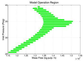
A final comment about this result, regarding to closed-loop behaviour, stands out the smart movements that a controller must execute in order to reject disturbances. For example, if operating point is  and a disturbance moves current point to , any controller movement must stay over the feasible region. Moving hydrocyclone inlets out of feasible region will produce abnormal operative condition, including equipment obstruction in one of output currents. In this sense, a single PID controller is not able to maneuver over the feasible region. To reach such closed loop operation, an additional structure must be design to coordinate PID actions. Therefore, a model for hydrocyclone as the presented in this work will be the core of a multivariable control structure. In this way the instrumentation and control area of mineral processing plants has a new tool to improve the process control.

4. Conclusion

A proposed model for hydrocyclone operation was presented and validated with data from a real assembly used for mineral processing. The modeling hypothesis is simpler compared with other approaches to the same modeling task, but results indicated usefulness of proposed model due to its low computational cost at good precision. Common mass conservation and mechanical energy balance (Bernoulli’s equation) was applied in order to cover the behavior of pulp inside the hydrocyclone. Through that approach, physical characteristics of overflow and underflow streams were predicted reaching a good agreement between experiments and model predictions. In addition, the inherent restriction caused over process inputs span when nonlinear behavior are included in process model was shown computing a hydrocyclone feasible operation region. This operation region showed that the input variables will produce a given set of operating acceptable values for model outputs. Out of this region, no meaning can be given to output values. Such a restricted zone is a consequence of nonlinearities acting as a whole to produce the complete process behavior.

Several future works must be executed in order to conform a final model: to verify using Computational Fluid Dynamics (CFD) the point of direction change from down overflow to up overflow, to propose a best split equation and to propose a better sub-model for air-core dimensions using CFD and video-supported images.

Acknowledgement

This work has been supported by COLCIENCIAS, project ID 47325, 633 Convocatoria Deducciones Tributarias año 2014.

References

[1] R. Venugopal and T. Chapperia, “Analysis and mathematical modelling of hydrocyclones - an overview,” in Proceeding of the International Mineral Processing Congress, 2012.
[2] Y. R. Murthy and K. U. Bhaskar, “Parametric CFD studies on hydrocyclone,” Powder Technology, vol. 230, pp. 36-47, 2012. View Article
[3] H. Schubert, “Which demands should and can meet a separation model for hydrocyclone classification?,” International Journal of Mineral Processing, vol. 96, no. 1-4, pp. 14-26, 2010. View Article
[4] M. Manninen, V. Taivassalo, and S. Kallio, “On the mixture model for multiphase flow,” 1996.
[5] C. Hirt and B. Nichols, “Volume of fluid (VOF) method for the dynamics of free boundaries,” Journal of Computational Physics, vol. 39, no. 1, pp. 201-225, 1981. View Article
[6] H. Alvarez, R. Lamanna, P. Vega, and S. Revollar, “Metodología para la Obtención de Modelos Semifísicos de Base Fenomenológica Aplicada a una Sulfitadora de Jugo de Caña de Azúcar,” Revista Iberoamericana de Automática e Informática Industrial RIAI, vol. 6, no. 3, pp. 10-20, 2009. View Article
[7] E. Hoyos, D. López & H. Alvarez, "A phenomenologically based material flow model for friction stir welding," Materials & Design, vol. 111, pp. 321-330, 2016. View Article
[8] Z.-B. Wang, L.-Y. Chu, W.-M. Chen, and S.-G. Wang, “Experimental investigation of the motion trajectory of solid particles inside the hydrocyclone by a Lagrange method,” Chemical Engineering Journal, vol. 138, no. 1-3, pp. 1-9, 2008. View Article
[9] K. Pana-Suppamassadu and S. Amnuaypanich, “Size Separation of Rubber Particles from Natural Rubber Latex by Hydrocyclone Technique,” in Proceedings of European Congress of Chemical Engineering (ECCE-6), 2007. View Article
[10] D. de Brito Dias, M. Mori, and W. P. Martignoni, “Study of Different Approaches for Modeling Cyclones Using Cfd,” in AIChE Annual Meeting, 2008. View Article
[11] K. Elsayed and C. Lacor, “The effect of cyclone height on the flow pattern and performance using LES,” in Tenth international congress of fluid dynamics (ICFD10), ASME, Egypt, 2010. View Article
[12] R. Darby, Chemical Engineering Fluid Mechanics, 2001. View Book
[13] W. B. Hooper, “The two-K method predicts head losses in pipe fittings,” Chemical Engineering, pp. 96-100, 1981.
[14] T. Neesse and J. Dueck, “Dynamic modelling of the hydrocyclone,” Minerals Engineering, vol. 20, no. 4, pp. 380-386, 2007. View Article
[15] S. Jayanti, “Bends, Flow and Pressure Drop in,” 2013, [Online]. Available: http://www.thermopedia.com/content/577