International Journal of Mining, Materials, and Metallurgical Engineering (IJMMME)

ISSN: 2562-4571

1. Introduction

In contrary to the traditional Discounted Cash Flow Method (DCFM), the Real Option Method (ROM) gives more flexible options. Since the study reported by Brennan and Schwartz [3], the application of ROM for estimating mining projects has been expanding in the theory and practice. Davis [5, 6] presents that the option premium can explain the gap between DCFM value and market value and the equations to estimate the volatility and dividend yield parameters to value real options. And many studies introduce ROM into natural resources investments such as Antonio and Dias [1], Dimitrakopoulos and Sabour [7], Guj [8], and Haque et al. [9].

However, regardless of commodity price, DCFM is still broadly used for project evaluations, especially in Korean mining investment projects. Although South Korean companies may have financial support from their government, many of them are reluctant to engage in mining projects because of uncertainty of business environment, such as commodity price volatility. In spite of the volatility, they still use DCFM to value mining projects in foreign countries, so that they cannot have the flexibility to make a decision to expand or postpone under uncertainty.

Thus, the main purpose of this study is to introduce ROM into a coal mining project in which Korean companies participate to justify the utility of ROM.

The paper is organized as follow: Section 2 presents shortcoming of DCFM as a traditional evaluation method, and propose ROM as a better alternative; Section 3 re-evaluates an investment of a coal mining project using both ROM to DCFM; Section 4 provides the necessity of ROM to evaluate oversea mining projects based on the result of ROM evaluation.

2. Discounted Cash Flow Methods and Real Option Method

2.1. Discounted Cash Flow Method – Static NPV

DCFM is commonly used to evaluate domestic and oversea South Korean mining projects. The technique of DCFM estimate the future new cash flows generated over the entire project life cycle using annual single-point forecasts of production and economic variables, such as future mineral commodity prices, production amounts, ore grade, recovery rate, consumable prices, and labour. These forecasts are used to construct an annual expected project new cash flow equal to revenue less capital and operating costs, government and third royalties, corporate income taxed, transport costs, insurance, and other deduction. Then this expected net cash flow is used to calculate a project Static Net Present Value (NPV) as an indication of project viability. The calculation of NPV requires estimating net annual cash flows and then discounting each annual cash flow for the value effects of uncertainty and time to determine a cash flow present value. NPV is the sum of these present value

CFt : Net Cash Flow during the period t
r : Discount Rate
I₀  : Total initial investment costs
t : number of time periods

The value effect of uncertainty and time is recognized by summarizing their impact into a single constant risk-adjusted rate that is used in the discounting process. This discount rate is likely used for a broad class of investment projects regardless of the actual uncertain characteristics of the particular project.

Although NPV method has been used widely in mining projects, it has shortcomings in its calculation process as follows. First, the use of a single discount rate implies that project cash flow uncertainty increases through time in a regular manner. However, most mine valuation professionals would agree that the cash flow uncertainty changes in a dynamic and erratic manner due to changes in mineral grades and prices, operating costs, mining method, exhaustion of tax shields, and tax and royalty rates among other things. Second, NPV method ignores the effects of contingent cash flows and flexibility. In the life of projects, volatility of mineral commodity prices may lead change of production policy, sliding scale royalty rates, and eventually change of cash flow structure. So, a risk adjustment method that responds to changes in cash flow uncertainty would be preferred.

2.2. Evaluation of Investment in Real Option Methods

The ROM approach considers multiple decision pathway as a consequence of high uncertainty coupled with flexibility in choosing optimal strategies or options along the way when new information becomes available. That is management has the flexibility to make midcourse strategy correction when there is uncertainty involved in the future. As information becomes available and uncertainty becomes resolved, management can choose the best strategies to implement. DCFM, static NPV, assumes a single static decision, while ROM assumes multidimensional dynamic decisions, where management has the flexibility to adapt given a change in the business environment. That is, ROM provides additional insights beyond DCFM. So, using ROM approach, an expanded net present value (NPV) can be calculated that includes static NPV determined from a conventional DCFM analysis plus an option premium that reflects the value of strategic options [11].

Expanded NPV = Static NPV + Option premium

• Expanded NPV: Value of investment using ROM
• Static NPV: Value of conventional DCFM
• Option Premium: Value of strategic options (management flexibility) in uncertainty

Standard option pricing models that explain the value of an option can be divided into a continuous time model and a discrete time discrete time model. One is the Black-Scholes model [2] and the other one is the Binomial tree model [4].

2.3. Black-Scholes Model and Binomial Tree as a Framework of ROM

Black-Scholes model

Black-Scholes developed the first mathematical model of pricing European Call options by using the following equation.

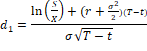
Where, C: call option value, P: put option value

S: underlying asset price, X: exercise price
r : risk free rate,  σ : volatility of underlying asset
T: time to expiration, t: time t
N(d): normal cumulative distribution function

The Black-Scholes model is comprised of a risk-free portfolio where returns can be represented by the risk-free rate. One crucial hypothesis of the model is the possibility to replicate the option with the underlying and a bond. This means that the holder of the option holds at the same time a portfolio that is designed to eliminate the risk stemming from the option. And the model assumes following [10]:

1. The risk-free rate is known and constant over time;
2. The asset pays no dividends;
3. The option can only be exercised at the maturity date;
4. There are no transaction costs when buying or selling an asset or derivate;
5. It is possible to invest any fraction of assets or derivate to the risk-free interest rate;
6. There are no penalties when short-selling is made;
7. The model is developed from the concept that the option asset price has a continuous stochastic behaviour, defined by the Geometric Brownian Motion (GBM)

Binomial tree model

Within comparison to the Black-Scholes model, the Binomial tree model allows the holder of an option to decide whether it is most beneficial to exercise the option or to wait until its maturity date, at each step. In addition, the model can calculate not only European options but also American options [12]. Also, the Binomial tree model converges to the Black-Scholes model when t in equation (2) is divided into more and more subintervals and r^f, u, d and q are used in such a way that the multiplicative binomial probability distribution of underlying asset prices goes to the lognormal distribution [4].

This Binomial tree model assumes that the maturity date of an option can be divided in discrete periods, whose dimension will be represented by δ^t.  Additionally, the price of the underlying asset is subject to a given behavior, and it will be multiplied by a random coefficient U or D, at each period (δ^t). It may be noted that random coefficients are defined as the price variation rate of the underlying asset. Since this rate can be ascending (U) or descending (D), reflecting the favorable or unfavorable market conditions, these multiplicative factors are dependent on volatility (σ) and length of the periods (δ^t). Figure 1 presents a binomial tree for the underlying asset, illustrating its price evolution. The nodes at the right represent the distribution of possible future values for the underlying asset.

The multiplicative factors, (U), probability of price increase and (D), probability of price decrease, are given by:

The probability of the asset price to increase or to decrease is given by a risk-neutral measure. Therefore, the asset price increases with a probability equal to:

and decreases with a probability given by:

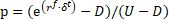
After determining these parameters, the option value can be obtained through a binominal tree. In this tree, each gain obtained for the underlying asset price is represented. For the case of a call option, this value is given by the maximum difference between the value of the underlying asset and its exercise price, and zero, i.e. max (S-X, 0). For the case of a put option, the value corresponds to the maximum difference between the exercise price and its asset price, and zero, i.e. max (X-S, 0). From the option value given by the nodes at the right of the tree, it is possible to calculate the other values applying the neutral probability on each pair of vertically adjacent values. They are mathematically represented by the following equation:

Where, Cn: the option value at node n

 

p: risk neutral probability
SUⁿ the asset value at node by probability of price increase
SDⁿ the asset value at node by probability of price decrease
r^f: risk free rate

In general binomial lattices are much more versatile and user-friendly than the Black and Scholes formula and can be effectively used in many circumstances [8]. So, this study uses the binomial tree model to estimate the value of a coal mining project.

3. The Case Study of Korean Bituminous Coal Mining Project

3.1. Summary of the Bituminous Coal Project

The Korean consortium is engaged in the project to utilize 3million tons of annual total bituminous coal production. There are four open pit mines and seven underground mines in the project site. The proved reserves of open pit mines and underground mines are estimated 40 million tons and 44 million tons, respectively (Table 1).

Table 2 presents the cash flow over the project’s life. The mine development period is from 2007 to 2009 and the mine production life is approximately 20 years starting 2009. Negative net after tax cash flows are expected for the development period (from 2007 to 2009). The NPV value of the project is estimated to be $ 1,318 million.

One of the open pit mines will start to operate at the first year of production, and subsequently other open pit mines will be phased in. The start of production in the underground mines is depended on business environment because of the low grade and the high cost in comparison to open pit mines in the project.

Table 1. Reserve of open pit mines and underground mines.

	Reserve		Resources	Planned life of production
	Proved	Probable
Open pit	40 mil ton	237 mil ton	407 mil ton	20 years
Underground	44 mil ton	35 mil ton	300 mil ton	-
Total	84 mil ton	272 mil ton	706 mil ton	20 years

Table 2. The cash flow of the project.
unit: K USD

	2007	2008	2009	2010	2011	2012	2013	2014	2015	2016	2017
Total Sales Revenue		0	0	318,162	761,441	699,172	740,128	779,187	770,878	639,724	635,780
Total Capital	18,000	390,000	1,000	1,000	18,000	13,000	48,000	26,000	4,000	48,000	4,000
Net Mine Operating Costs		0	16,740	159,468	281,432	273,751	317,750	350,069	345,806	327,386	354,195
Tax			-10,737	42,238	138,468	121,701	119,348	120,590	119,257	83,996	75,025
Working Capital		0	2,064	-8,554	-21,397	4,171	-15,514	-1,698	1,575	14,189	3,629
Net After Tax Cash Flows	-18,000	-390,000	-9,067	124,010	344,939	286,549	270,543	284,226	300,240	166,152	198,930
	2018	2019	2020	2021	2022	2023	2024	2025	2026	2027	2028
Total Sales Revenue	653,255	653,255	643,806	613,559	613,559	613,559	613,559	613,559	613,559	613,559/td>	613,559
Total Capital	48,000	18,000	4,000	48,000	5,000	48,000	18,000	5,000	5,000	5,000	-58,000
Net Mine Operating Costs	347,812	343,843	322,091	313,313	335,192	356,355	370,743	372,436	364,820	364,820	364,820
Tax	81,118	81,769	84,994	77,279	70,955	64,606	60,530	59,992	63,567	63,162	49,167
Working Capital	-3,044	2,556	-2,129	1,404	2,697	2,609	1,774	209	-939	0	0
Net After Tax Cash Flows	179,369	207,087	234,850	173,564	199,714	141,989	162,512	175,922	181,112	180,578	257,573

* Discount rate: 9%

3.2. Valuation of the Project ROM

The valuation of the project by NPV assumes only development and production of open pit mines at the first stage and does not include any cost and revenue of underground mines which could start operation in accordance with changes of market environment. Thus, this study assumes that underground mines would be developed and operated allowing for the market environment to value the project using option to expand, one of real options.

3.2.1. Estimation of Parameters for ROM

Estimation of volatility of bituminous coal price

Estimation of volatility in real option valuation techniques is calculated based on past movement of the asset price or revenues, otherwise it is estimated by simulating the future predicted revenue. But, this study chooses monthly Australian coal prices (New castle FOB) from Jan. 2002 to Nov. 2010 by applying the first difference of log and estimates the monthly standard deviation. For the transition to the annual standard deviation, the estimated monthly standard deviation is multiplied by . Then, it is obtained the annual standard deviation 29.91% is obtained (Table 3).

Table 3. Error rates for four different trials.

Monthly average	1.26%
Monthly standard deviation	8.64%
Annual average	15.17%
Annual standard deviation	29.91%

Underlying asset value (S)

The value of NPV which is already calculated as cash flow analysis of the project plus the amount of investment is the underlying asset value of the project (Table 4).

Table 4.Underlying asset value.
unit: M  USD

Investment(A)	NPV(B)	Underlying asset value S = A + B
409	1,318	1,727

Maturity(T) and Exercise price(X)

The expiration of the expansion option is assumed in fifth year when production from underground mines is started. And the exercise price of the option is $263,387, investment to develop underground mines.

Expansion Factors (E^f)

If open pit mines and underground mines are operated together, total amount of production in the project is increased by 1.36 times compare with the production from open pit mines only (Table 5).

Table 5. The total amount of production in the project.

	Open pit mines only (K USD)	Expansion (Open pit mines+ Underground mines) (K USD)	The rate of increase in production amounts (%)
Total amount of production	162,479	220,661	1.36

Probabilities of ascending coal price and descending coal price (U & D)

Probabilities of ascending coal price , and descending coal price . Using two equations, the probability of ascending coal price , the probability of descending coal price = 1/1.349= 0.741.

Risk-free rate (r^f)

It is 2.66%, which is the return rate of US Treasury bonds with a maturity of 10 years at Nov, 1, 2010.

Risk neutral probability (p)

The risk neutral probability is 0.470 result in substituting the values of probabilities of ascending coal price and descending coal price into the equation of risk-neutral probability, .

3.2.2. Valuation by the Expansion Option

Table 6 shows the possible evolution of the underlying asset price(S) from the left to the right using probabilities of ascending coal price and descending coal price. And it is necessary to calculate using recursive backward iteration to estimate the option value on the basis of the value of underlying asset.

The calculation of the investment value at the maturity date is to select the greater value between the exercise value and the maintain value. For example, the investment value, including the expand option, at the maturity date, SU⁵, is as follows.

Table 6. Evolution of the underlying asset of the project using the binomial distribution model.
unit: M USD

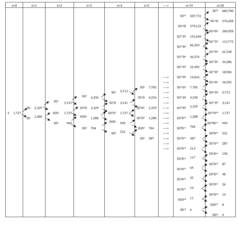
Table 7. Evolution of the value of the project by an expand option and the decision tree.
unit: M USD

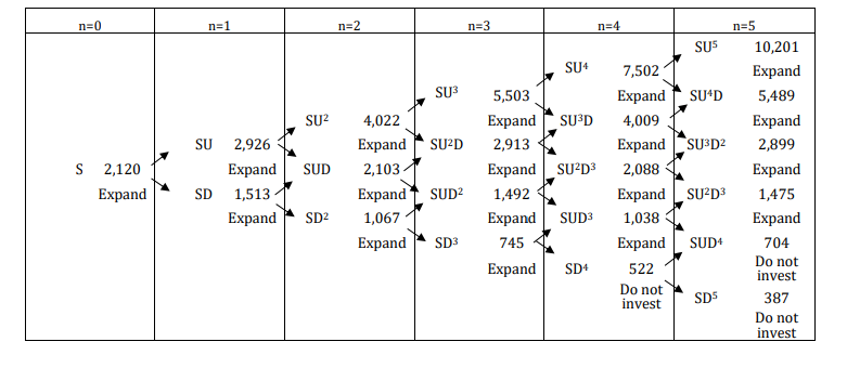
Table 8. The value of the project by the expand option.

	Value (M USD)	Refer
A_ underlying asset value	1,727	Underlying asset S
B_ Option value of underlying asset	2,175	Option value of underlying asset S
C_ the value of option	449	B - A
D_ NPV	1,318	Value of the project using NPV
Expanded value of the project	1,766	C + D

Since the expansion investment of, $10,201 million, is greater than the underlying asset value of $ 7,705 million at SU⁵ node, the expansion option has to be exercised to invest. But the expansion option cannot be exercised at SD⁵ node because the value of expansion investment is lower than the value of underlying asset.

The value from SU⁴ node, using the risk-neutral probability, is inversely calculated from the maturity time of expansion options as follows

The value of the expansion option is larger than the value of the underlying asset at SU⁴ node, so the optimal decision is to expand the project. The optimal decision and the option value at each node are showed in Table 7 through the calculation as described above. Table 8 shows that the value of the project by expansion option is US$ 1,766, which is higher than the NPV value (US$ 1,318). The expansion option value is given by difference between the static NPV and the expanded NPV. Thus, the Korean consortium should prepare to invest more when they face the favorable investment conditions such as global coal price surge.

5. Conclusion

Traditional DCFM such as NPV does not provide the optimal time to invest and the true value of project in uncertainty. However, ROM is a methodology used to evaluate real assets that considers management flexibility over the project’s lifetime. As new information is considered and uncertainties are revealed, investors can estimate the final project value using ROM. The present  study re-estimates a Korean bituminous coal mining project using ROM and compares ROM with DCFM to prove that ROM has advantage under uncertain business environment.

Acknowledgments

This study was supported by the Research Program ‘Development of mineral potential targeting and mining technologies based on 3D geological modelling platform’ by KIGAM.

References

[1] M. Antonio, and G. Dias, “Valuation of exploration and production assets: an overview of real options models,” Journal of Petroleum Science & Engineering, vol. 44, no. 1-2, pp. 93-114, 2004. View Article
[2] F. Black, and M. Scholes, “The Pricing of Options and Corporate Liabilities,” Journal of Political Economy, vol. 81, no. 3, pp. 637-354, 1973. View Article
[3] M. Brennan, and E. Schwartz, “Evaluating natural resource investment,” Journal of Business, vol. 58, no. 2, pp. 135-157, 1985. View Article
[4] J. C. Cox, S. A. Ross, and M. Rubinstein, “Option Pricing: A Simplified Approach,” Journal of Financial Economics, vol. 7, no. 3, pp. 229-263, 1979.View Article
[5] G. Davis, “Option premium in mineral asset pricing; are they important?,” Land Economics, vol. 72, no. 2, pp. 167-186, 1996.View Article
[6] G. Davis, “Estimating volatility and dividend yield when valuing real options to invest or abandon,” Quarterly Review of Economic and Finance, vol. 38, no. 3, pp. 725-754, 1998.View Article
[7] R. Dimitrakopoulos, and S. A. Sabour, “Evaluating mine plans under uncertainty: Can real options make a difference?,” Resources Policy, vol. 32, pp. 116-125, 2007. View Article
[8] P. Guj, “A practical real option mythology for the evaluation of farm-in/out joint venture agreements in mineral exploration,” Resource Policy, vol. 36, no. 1, pp. 80-90, 2011. View Article
[9] Md. Haque, E. Topal, and E. Lilford, “A numerical study for a mining project using real options valuation under commodity price uncertainty,” Resources Policy, vol. 39, pp. 115-123, 2014.View Article
[10] L. Santos, I. Soares, C. Mendes, and P. Ferreira, “Real Option versus Traditional Methods to assess Renewable Energy Project,” Renewable Energy, vol. 68, pp. 588-914, 2014.View Article
[11] M. Samis, G. Davis, D. Laugton, and R. Poulin, “Valuing uncertain asset cash flows when there are no options: A real options approach,” Resource policy, vol. 30, no. 4, pp. 285-298, 2006.View Article
[12] L. Trigeorgis, “Real Options: Managerial Flexibility and Strategy in Resource Allocation,” MIT press, 1997.