International Journal of Mining, Materials, and Metallurgical Engineering (IJMMME)

ISSN: 2562-4571

1. Introduction

When designing the overall heat release rate of an object, calculating the appropriate ignition time of the various fuel packages will be decisive. During several earlier studies on the heat release rate of mining vehicles [1-2] the question on how the surface roughness will affect the ignition was raised. The environment in mining industries is distinguished by heavy tear and rough fuel surfaces. The surface roughness magnitude of the gauges, dents etc. could be substantial, where the roughness depth would range from less than a millimeter up to several millimeters. Treads on tyres found in the mining industry could be several centimeters in depth [3].

An important component when quantifying the spread and behavior of a fire is the ignitability of a fuel item, for example a tyre or a hydraulic hose on a mining vehicle [4]. Typically fuel item ignition characteristics are measured based on flat surfaces. Many fuel items have non-flat surfaces that can be characterized based on surface geometry using the concept of a surface roughness. How the surface roughness effects fuel item ignition is not well defined at this time.

Any surface protuberances on an uneven surface would ignite first; as these will be exposed by heat transfer from several directions as we are facing a two/three-dimensional ignition scenario. Heskestad [5] performed ignition tests on samples with variable surface roughness and found that the ignition time was largely affected by the surface structure for diffusion flames as well as premixed flames. Akita [6] performed ignition tests on wood with variable surface roughness and found no differences in ignition time. These two studies point in different directions but the number of experiments in the papers was limited and the subject has not been investigated to any larger extent.

The work presented consists of an analysis where results from cone calorimeter experiments and a twodimensional analysis were used for exploring potential relationships with respect to the ignition of rough fuel elements. The aim and purpose of this paper is to perform an exploratory analysis on the influence of surface roughness with respect to ignition that may act as a basis for future studies. Besides surfaces characterized by roughness, the results may also be applicable to non-flat surfaces where the surface structures are part of the design of the equipment such as tyre treads.

2. Theory

2. 1. Defining surface roughness parameters

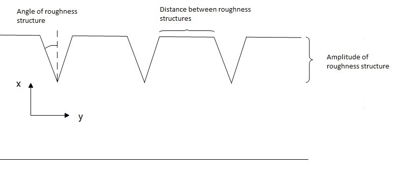
Surface roughness can be distinguished by the random nature and found in two dimensions. Perpendicular to the surface the height of the protuberances can be distinguished. Parallel to the surface the texture of the protuberances can be distinguished [7]. Interesting parameters in order to characterize the roughness of a surface would thus be the amplitude and the distribution of the protuberances.

The features of surface roughness can be described in numerous ways. Due to the random nature of the protuberances an average value of the specific parameter is often best suited when characterizing the surface roughness. The following parameters are examples of average values:

- Amplitude of roughness structures to get a picture of the vertical characteristics of the surface structure. This could be defined as the average absolute deviation of the roughness structures from the mean line:

Where R_a is the average height (m) and x is the distance to point of interest (m).

- Distance between roughness structures to get a picture of the horizontal characteristics. This could be described by the average distance between local peaks:

Where S is the mean distance between adjacent peaks (m).

- The slope or angle of the roughness structure will provide a picture of the combination of the vertical and horizontal characteristics. This could be described by average absolute slope of the roughness structure:

Where is the average absolute slope (degree) and is the slope of the roughness structure (degree).

The three parameters above represent the three groups that surface roughness structures are normally divided into: amplitude parameters, horizontal distance parameters and parameters representing a combination of amplitude and horizontal distance parameters. In the ensuing two-dimensional analysis and cone calorimeter experiments gauges with certain angles, depths and distances were applied in order to depict roughness features. In Figure 1 the parameters are described for a two-dimensional cross-section of a specimen. The simplified surface roughness features and the milling of the structures were performed to obtain controlled and homogeneous structures suitable for an exploratory analysis.

2. 2. Ignition process

Ignition of a fuel item will depend on its flat surface reaching a critical condition such as a temperature. The ignition temperature represents the point in time when a flat surface can support flaming ignition [8-9]. For this critical condition to be reached, the incident heat flux must exceed the surface losses at the ignition temperature. Surface roughness will then be expected to affect the local incident heat flux and the local surface losses. In turn the local temperature would be expected to vary based on the characteristics of the roughness.

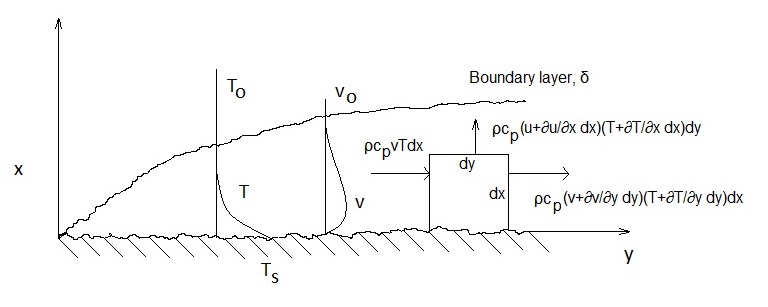
Figure 2 depicts the ignition process at a rough surface where the fuel sample has a horizontal orientation and the mass flow in the direction of the heat source. In the case of a vertical fuel sample orientation the physics will different, also a forced flow will present a different situation as opposed to the buoyantly generated flow seen in Figure 2.

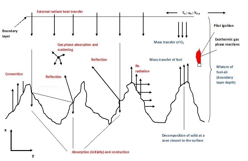
In the following the two-dimensional governing equations for the solid/gas interface for a rough horizontal surface exposed to radiant heating are presented and discussed. The presented models are primarily based upon the one-dimensional models of Atreya [8]. In the analysis and experiments only the piloted ignition is accounted for, as the piloted ignition was used at the cone calorimeter tests. The governing equations of the gas phase and the solid phase can be found for example in a paper by Atreya [8].

2. 2.1. Governing equations of the solid/gas interface

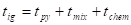
Quintiere [10] presented an expression containing the individual ignition time components:

Where is the time to ignition (s). The -component describes the time to attain the temperature where adequate fuel vapor concentrations are emitted. The -component accounts for the time needed for fuel vapors and oxygen to reach the ignition source. The -component accounts for the time from when the flammable mixture reaches the ignition source until combustion. The focus will be on the - and the -component as these will dominate over the -component (negligible where strong ignition conditions prevail which can be assumed for the experiments).

Initial boundary conditions () within the boundary layer ():

Where is the mass fraction of fuel,  is the mass fraction of oxygen, is the mass fraction of oxygen in the ambient air,  is the temperature (K) and is the ambient air temperature (K).

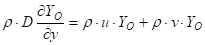
Fuel conservation at the surface (), :

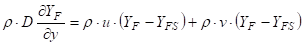
Where  is the density (kg m^-3),  is the diffusion coefficient (m² s^-1),  is the distance to point of interest (m),  is the gas velocity in the x-direction (m s^-1),  is the mass fraction of fuel in the volatiles and  is the gas velocity in the y-direction (m s^-1).

Oxygen conservation at the surface, :

Fuel temperature at the surface, :

Where  is the surface temperature (K).

Boundary conditions at the boundary layer  (), :

Where is the heat flux (kW m^-2),  is the external incident heat flux (kW m^-2),  is the emissive power of cone calorimeter (kW m^-2),  is the view factor between cone calorimeter and the boundary layer, and is the transmissivity of air.

Assuming optically thin conditions, the gas phase absorption of radiation can be neglected and the heat flux from the cone calorimeter can be expressed as:

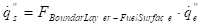
Where  is the heat flux at fuel surface (kW m^-2) and  is the view factor between the boundary layer and the surface of the fuel.

The heat flux from the cone is measured at the surface which strengthens the neglecting of the gas phase absorption.

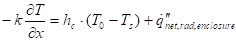
The solid boundary condition at a surface plane:

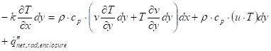
Where  is the thermal conductivity (kW m^-1 K^-1),  is the specific heat (kJ kg^-1 K^-1) and  is the net radiation term for upper surface () (kW m^-2).

The temperature change in the y-direction is assumed to be small and the conduction in the flow direction is negligible. The net radiation to the solid surface is the final term on the RHS of the equation and is solved through a network analysis described below.

The temperature continuity at the interface:

Where  is the fluid temperature (K).

The heat flux continuity (no-slip condition):

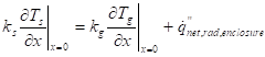
Where  is the thermal conductivity of solid (kW m^-1 K^-1) and  is the thermal conductivity of fluid (kW m^-1 K^-1).

Figure 3 displays the natural convection case and the convective energy flows of a control volume at the interface. The resulting second-order differentials of the convective energy were neglected in equation (16).

Given that the mixing time is small compared with the heating time - see below for analysis - the gas phase details can be simplified with respect to the mixing time, where a heat transfer coefficient is used in equation (16):

Where  is the convective heat transfer coefficient (kW m^-2 K^-1).

To investigate the gas phase flow field over the solid surface, the boundary layer thickness was calculated for two cases: forced flow and natural convection over a horizontal specimen facing upwards.

For the forced flow case, the boundary layer thickness was calculated based upon the Reynolds number resulting in a laminar flow case [11]. Figure 4 displays the boundary layer thickness as a function of the distance from the edge of the specimen.

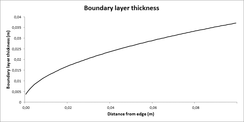
For the natural convection case, the boundary layer thickness was calculated applying a paper by Lewandowski et al. [12]. The model assumes that the thermal and hydraulic boundary layers have comparable thicknesses.

The equations for the two cases are valid for flat surfaces and the boundary layer thickness for a surface with milled gauges will not be identical. Nevertheless, the equations are applied in order to obtain approximate values. Given the boundary layer thickness, the mixing time was calculated applying a binary diffusion coefficient for carbon monoxide. The mixing time above the centre of the specimen for both cases was found to be small in comparison with the ignition times of the experiments and therefore the gas phase details can be simplified with relation to the mixing time.

The spark igniter in the experiments is located 13 mm above the centre of the specimen, which is within the boundary layer for both cases. This will imply that no additional transport time beside the mixing time should be considered and piloted ignition prevails.

In the two-dimensional analysis the following assumptions were made:

-              Heat losses due to moisture content of the fuel sample are neglected, assuming low moisture content.

-                 The fuel decomposition will occur in depth of the fuel sample and charring is assumed.

-                 The mass flux is low prior to ignition and the heat of pyrolysis is neglected.

-                 An opaque material is assumed as well as gray and diffuse fuel surfaces.

-                 The gas of the boundary layer is a non-participating gas as the optical pathlength will be small due to the short distance between the cone element and the specimen. The optical pathlength of the non-participating gases was calculated for two cases using a physical pathlength of 0.0025 m and 0.0030 m and the mean absorption coefficient [13] of the gases at 663.5 K (average temperature at ignition). The optical pathlengths were <<1 and thus fulfilling the optical thin case criterion.

-                 The radiation is absorbed at the surface.

-                 The infinitely thin surface of the sample with virtual sides representing the boundary layer and the ambient above the boundary layer is regarded as an enclosure when accounting for the radiative heat transfer from the cone to the interface.

The contribution of the gas-phase exothermic reactions is negligible in the energy balance at the interface.

2. 3. Network analysis

The following assumptions were made related to the network analysis:

- The temperature along a gauge surface and for an upper surface segment will vary and therefore the surfaces were divided into finite parts.

- For the gauges a three sided enclosure is assumed, consisting of the two gauge slopes and the upper virtual side - in level with the upper surface of the specimen.

- Uniform emissivity for the finite parts.

- The incident radiation upon the upper surface is set to 35 kW m^-2 at the centre of the specimen, equivalent to the measured heat flux at the specimen surface during the calibration procedure. This requires that the boundary layer gas is a non-participating gas.

The emissive power of the individual surfaces:

Where  is the emissive power of surface  (kW m^-2),  is the Stefan-Boltzmann constant (5.67·10^-11 kW m^-2 K^-4) and  is the surface temperature of surface  (K).

The radiative heat flow resistances:

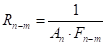
Where  is the radiative heat flow resistance between surface  and  (m^-2),  is the view factor between surface  and surface ,  is the radiative heat flow resistance of surface  (m^-2),  is the area of surface  (m²) and  is the emissivity of surface .

The individual net interchange between two surfaces:

Where  is the net heat flow from surface  to surface  (kW).

The net interchange between the cone and a surface ():

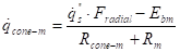
 describes the view factor along the surface and  is the radiative heat flow resistance between the cone calorimeter and surface  (m^-2).

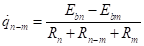
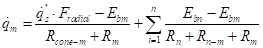
The individual net interchange terms for a surface are summed up into a total net heat flow:

The net radiation term of equation (19):

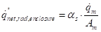
Where is the absorptivity of the fuel surface.

2. 3.1. View factors

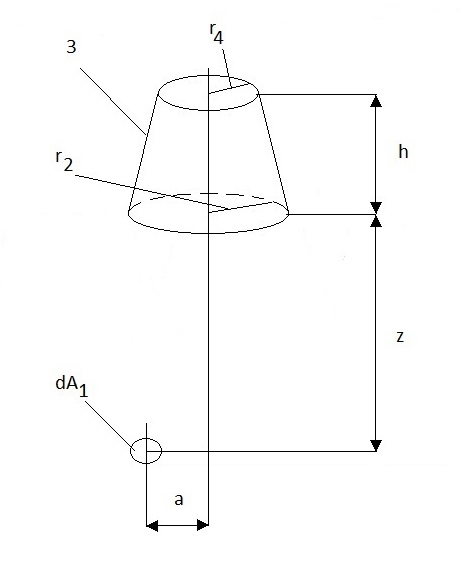
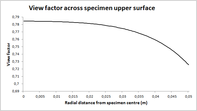
The variation of the incident radiation with the radial distance from the centre for an upper surface: The incident radiation varies with the radial distance from the centre and can be described applying [14]:

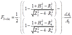
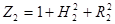
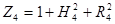
Where  is the view factor between the cone calorimeter surface and a surface element , is the cone calorimeter surface area,  is the radial distance between the centre of the cone calorimeter and the centre of the surface element  (m),  is the radius of cone (m),  is the height of cone (m) and  is the distance between cone calorimeter and upper fuel surface (m).

The parameters of equations (28-33) are seen in Figure 5.

Figure 6 displays the view factor across the upper surface as a function of the radial distance from the centre. In the calculations the view factor at the centre was set to 1 and the view factor of adjacent segments was adjusted accordingly.

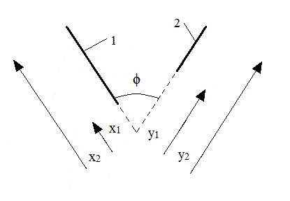
The view factor term in equation (21) can be differentiated into three cases:

a) Two infinitely long surfaces having a common edge with an included angle [15].

b) Two infinitely long surfaces of equal widths having a common edge with an included angle [16].

c) Two infinitely long surfaces without a common edge with an included angle [16].

a) Two infinitely long surfaces having a common edge with an included angle [15]:

Where  is the angle between two opposing surfaces with lengths  and  respectively and with a common edge (degree), and  is the view factor between surface  and.

The parameters of equations (34) and (35) are found in Figure 7.

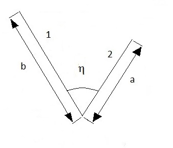
b) Two infinitely long surfaces of equal widths having a common edge with an included angle [16]:

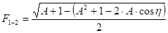
c) Two infinitely long surfaces without a common edge with an included angle [16]:

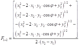
Where  is the angle between two opposing surfaces without a common edge (degree),  and  is the distance from the vertex to the inner edge of surface 1 and 2,  and  is the distance between the vertex and the outer edge of surface 1 and 2.

The parameters of equation (37) are found in Figure 8.

3. Experiments and two-dimensional analysis

3. 1. Cone calorimeter experiments

Cone calorimeter experiments were conducted in the Fire Science Laboratory at WPI.

The specimens were white pine boards (0.1x0.1x0.025 m (LxWxH)) as the surface would not change shape during the pre-ignition phase, exceeding the length scale of the roughness structures. Even though tyre or hose samples were not used in the experiments, wood is also a fuel that can be found in the mining industry (for example wooden pallets, sheds or boards preventing tear on electrical cables). Measurements were performed to verify thermally-thick behavior.

V-shaped gauges were milled in the same direction as the grain - depicting roughness features - varying the depth, angle and distance; see Table 1 and Figure 1. Table 1 also includes the normalized characteristic lengths of the cases, with respect to the width/length of the cone specimen (i.e. 100 mm). The limited data set was due to the scoping study nature of the project.

Case #1 had no roughness feature for reference. Throughout the experiments the incident heat flux was set to 35 kW m^-2.

Several experiments were also conducted with a heat flux of 50 kW m^-2, but the increase in heat flux resulted in virtually no differences in ignition time between the experiments.

The ignition time, temperature on upper surface and in a gauge (using glass braid insulated thermocouples with 0.25 mm diameter and a 2.2°C tolerance) were recorded. The thermocouples in the gauges were positioned in the upper third part of the gauge as it was difficult to position the thermocouples at the bottom.

The average specimen moisture content was measured at 5.8%, using a P-2000 electrical resistance-type moisture meter from Delmhorst Instrument.

Outlier elimination of ignition times and surface temperatures were conducted as single values stood out. When outlier elimination was applied the change in the average value was minimal.

When looking into the temperature data of the cone experiments it was noticed that when the shutter opened a sudden temperature increase occurred followed by a period where the temperature levelled out and finally a rapid temperature increase. An ignition criterion was defined in this paper as the point of time when the temperature initiated this final and sudden increase.

3. 2. Finite Difference Method

A two-dimensional analysis – applying a finite difference methodology – of the heat conduction into the specimen was conducted, varying:gauge depth, angle and distance. Table 2 lists the different cases, identical with the experiments.

Unsteady-state conduction and no energy generation were assumed. Neglecting heat of pyrolysis and assuming an opaque material, the energy equation of the solid phase:

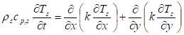
was applied. Where  is the density of solid (kg m^-3) and  is the specific heat of solid (kJ kg^-1 K^-1).

The exposed face solid boundary condition of equation (19) was applied as well.

The roughness parameters can be linked to equation (19). The convective heat transfer, first term on right hand side of equation (19), is assumed constant relative to the surface roughness due to the “shallow” normalized depths (up to 5%).  The radiation heat transfer, second term on the right hand side of equation (19), accounts for the changing aspects of the surface roughness. It is assumed that the incident radiation to each node varies with the radial distance from the centre of the specimen. It is also assumed that the incident radiation inside a gauge enclosure will vary with the gauge angle and depth.

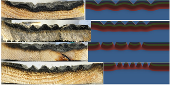
Figure 9 displays the node set-up in two cases; the upper case has a 2 mm gauge depth, 45° gauge angle and 10 mm gauge distance, the lower case a 5 mm gauge depth, 60° gauge angle and 2 mm gauge distance. The blue squares represent interior nodes, the red represent surface nodes, the orange exterior corner nodes and the green interior corner nodes.

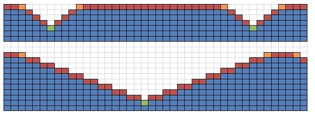
Each upper surface node shown in Figure 9 exchanges radiation with the ambient environment only. Each surface node that is part of a gauge, see Figure 9, exchanges radiation with the ambient and the other parts of the gauge that can be “seen” from the given node.  A virtual enclosure is established for each gauge based on its characteristics and the appropriate view factors are calculated to establish the radiative exchange “within” the virtual enclosure.

3. 3. Set up of two-dimensional analysis

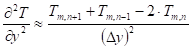
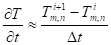
Unsteady-state conduction and no energy generation were assumed in the analysis. Neglecting the heat of pyrolysis and assuming an opaque material, the energy equation of the solid phase (equation (38)) is applied where the second partial derivatives and the time derivative are approximated by:

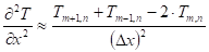
Where  is the interior node temperature (K),  is the interior node temperature with one distance increment added in the x-direction,  is the interior node temperature with one negative distance increment added in the x-direction,  is the interior node temperature with one distance increment added in the y-direction,  is the interior node temperature with one negative distance increment added in the y-direction,  is the interior node temperature at time step  (K),  is the interior node temperature at time step  (K),  is the time increment (s),  and  are distance increments (m).

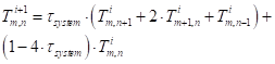
Inserting the approximations into equation (38) results in the following approximation for an interior node:

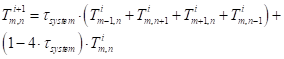
Where  is the time constant of the system (s) and  is the thermal diffusivity (m² s^-1).

Figure 10 displays an interior node system.

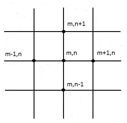
The solid boundary condition at a surface plane (equation (19)) can be approximated by the following approximation for a surface node (setting the energy conducted, convected and radiated into the node equal to the internal energy increase of the node):

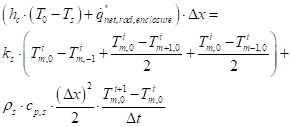
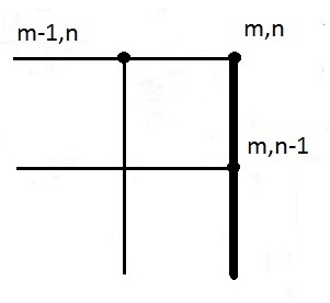
Where node temperature parameters containing a 0 in the subscript indicates a surface node. For an upper surface node, the heat flux term on the LHS of equation (45) only contains the net interchange between the cone heater and the surface node. See Figure 11 for the node system.

The approximation of equation (19) for an exterior corner node:

The first term on the LHS of equation (46) only involves the net heat flux term from cone calorimeter to the upper surface of the corner node. The second term involves both the net heat flux term from cone calorimeter to the slope segment and the net interchange term of the slope segment. See Figure 12 for the node system.

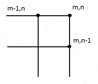
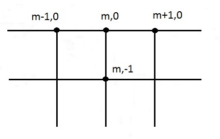
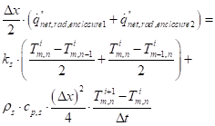
Approximation of equation (19) for an interior corner node:

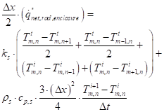
See Figure 13 for the node system.

Approximation of equation (19) for an exterior corner node with one side insulated:

For a corner node along the upper surface, the heat flux term on the LHS of equation (45) will only contain the net interchange between the cone heater and the surface node. See Figure 14 for the node system.

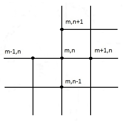
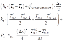
Approximation for an internal node - applying equation (19) - with one side insulated:

See Figure 15 for the node system.

Tabulated values for pine (moisture content of 0%) [9] were applied in the analysis:

-   Heat capacity: 1.8 kJ kg^-1 K^-1

-   Thermal conductivity: 0.185 W m^-1 K^-1

-  Density: 510 kg m^-3

A sensitivity analysis was carried out to find the optimal distance increment, applying [11]:

Based upon the results, the time increment was set to 0.25 s and the distance:  m.

The absorptivity and the emissivity of the white pine surface was assumed to be 0.88, as there were no experimental data available [9].

The convective heat transfer coefficient was set to 0.024 kW m^-2 K^-1, valid for a heat flux of 35 kW m^-2 in a cone calorimeter [9].

3. 4. Procedure of the model calculations

In order to further clarify the model details, the step-by-step procedure is presented here:

The first step involved setting up the geometry of the specific case and dividing the sample into the different types of nodes with the optimal distance increment. Initially the temperature of the gauge and upper surface nodes were set to the same temperature as the thermocouples recorded when the shutter was opened.

During the second step the view factors for the different surface nodes were calculated using expressions described above, both with respect to the cone heater as well as for nodes facing each other in the gauges.

The third step involved using equation (19) and applying the external heat flux from the cone heater and the surface temperature of the previous time step, the incident heat flux at the various surface nodes were calculated. The net interchange term for a gauge surface node was calculated using equation (25) and for an upper surface node equation (24) was used. In both cases the emissive power of the individual surface nodes were calculated applying the surface temperature from the previous time step.

In the fourth step the temperature of the surface nodes as well as the internal nodes were calculated applying the different approximate equations described above as well as the node temperatures from the previous time step.

The calculations are repeated for the third and fourth step for each time step.

Table 1. The configuration of each experimental case; resulting ignition times and temperatures of the experiments.

Case #	Depth of gauges (mm)	Angle of gauges (degrees)	Distance between gauges (mm)	Number of Gauges	Normalized depth	Normalized distance	Average ignition time (s)	Standard deviation ignition time	Average upper surface temperature (°C)	Standard deviation upper surface temperature	Average gauge temperature (°C)	Standard deviation gauge temperature
1	0	0	0	0	0	0	30	2	364	20	-	-
2	2	45	10	5	0.02	0.1	34	2	404	18	384	10
3	5	45	10	4	0.05	0.1	411	2	4112	16	3713	20
4	2	45	2	9	0.02	0.02	30	2	346	25	365	13
5	5	45	2	5	0.05	0.02	401	4	360	20	356	12
6	2	30	10	5	0.02	0.1	26	2	370	23	346	25
7	5	30	10	4	0.05	0.1	31	3	377	40	31434	20
8	2	60	10	4	0.02	0.1	171	1	3132	22	3004	14
9	5	60	10	3	0.05	0.1	30	4	363	20	345	16
10	2	30	2	8	0.02	0.02	26	1	361	14	359	25
11	5	30	2	6	0.05	0.02	351	4	364	16	336	29
12	2	60	2	6	0.05	0.02	31	3	361	19	368	18
13	5	60	2	4	0.05	0.02	28	2	344	15	353	20
14	2	30	20	3	0.02	0.2	251	1	390	6	3363	16
								Avg = 2		Avg = 20		Avg = 18

¹ Shows significant difference based on 1 SD variation (4 sec) compared to Case #1 for ignition time.

² Shows significant difference based on 1 SD variation (40 °C) compared to Case #1 for upper surface temperature.

³ Indicates significant difference based on 1 SD variation (38 °C) between upper surface and gauge temperatures.

⁴ Shows significant difference based on 1 SD variation (36 °C) compared to Case #1 for gauge temperature.

4. Results and discussion

Establishing a significant difference between the mean experimental values, a criterion where the range of one standard deviation of the means did not overlap each other was applied, see Table 1. 

4. 1. Ignition times of experiments

Table 1 displays the average time of ignition for all experimental cases. Five of the thirteen cases showed significant difference when compared to the flat surface case. These five cases did not show any clear pattern related to the gauge characteristics.

4. 2. Surface temperatures at ignition from experiments

Table 1 displays the average upper surface and gauge temperatures for all experimental cases.  Two out of thirteen cases for the upper surface temperature and two out of thirteen cases for the gauge temperature showed significant difference when compared to the flat case. These cases show no clear pattern related to the gauge characteristics. Comparing the upper surface and gauge temperatures for each case showed significant temperature difference in three out of thirteen cases. These cases show no clear pattern related to the gauge characteristics.

4. 3. Surface temperatures at t=25 s from two-dimensional analysis

Table 2 displays the average node temperatures at t=25 s from the two-dimensional analysis.  This fixed time will be used to verify the two-dimensional analysis. The point of time at t=25 s was selected as it was just prior to the ignition of most of the experiments and distinct temperature differences had been established at that time. The average upper surface temperature was the average surface node temperatures between two gauges in the centre of the sample. The upper 1 mm gauge slope temperature was the average surface node temperatures for a corner node and the corresponding nodes below it into the gauge for a distance of 1 mm. The average gauge bottom temperature was the node temperatures of the bottom node.  The location of both these temperatures was the gauge closest to the specimen centre.

The upper surface and upper 1 mm gauge temperature increase as gauge depth increases for all angles and spacing. This is consistent with the fact that the net difference between heating (incident heat flux from cone and re-radiation within gauge) and cooling (convective cooling and re-radiation out of the gauge) increases with increasing depth.

The gauge bottom temperature decreases as the gauge depth increases for all angles and spacing. This is consistent with the fact that the view factor from the cone heater to the bottom node always decreases with increasing depth and the view factor from opposite gauge slope to bottom node also decreases with increasing depth.

The upper surface and upper 1 mm gauge temperatures decrease as gauge spacing increases for all angles and depths - except the 30° cases with a 2 mm gauge depth. This is consistent with the fact that the temperatures of the edge nodes are generally higher than the upper surface temperature as the edge node is exposed to heat flux from two directions. With increasing gauge distance between edge nodes, the upper surface temperature will decrease as edge node heating effect decreases. With a longer distance between two edge nodes, the cooling effect of the upper surface will increase and result in lower upper 1 mm gauge temperatures. The edge node temperatures in the 30° and 2 mm depth cases are lower than the upper surface temperatures as the net difference between heating and cooling is lowest for the 30° cases.

The gauge bottom temperature decreases or does not change as gauge spacing is increased for all angles and depths - except for the 30° cases. This is consistent with the fact that variations of the gauge distance will influence the upper nodes and upper surface but not the gauge bottom to the same degree. In the 30° cases - as the edge node has a lower temperature - an increasing spacing will result in higher upper surface temperature which will affect to some extent the gauge bottom temperature.

The upper surface, the upper 1 mm gauge and gauge bottom temperatures all increase with increasing gauge angle for all depths and spacing. The upper region temperature increase has a peak at a gauge angle of 60° for the 2 mm depth and at a 45° angle for the 5 mm depth. This is consistent with an increase in the surface area and that the net difference between heating and cooling increases as the gauge angle increases. As the depth increases a larger portion of the radiative energy is re-radiated from nodes in the upper slope region to the lower nodes in the 60° case than for the 45 or 30° cases.

Given the results of the model at t=25 s, the output of the model was found to be consistent with the definition of the boundary conditions and the virtual enclosures for the gauges.

4. 4. Surface temperatures at ignition from two-dimensional analysis

Table 2 displays the average temperatures at the time of ignition from the two-dimensional analysis.

The upper third gauge slope temperature was calculated for comparison with the experimental results as the thermocouples in the gauges were positioned in this part of the slope. The upper third gauge slope temperature was the average surface node temperatures for a corner node and the corresponding nodes below it into the gauge for one third of the total slope length. The location of the temperature was the gauge closest to the specimen centre. The upper surface and gauge bottom average temperatures are defined the same as previously noted for the t=25 s discussion.

The significant difference of the model was defined as the level of significance of the experimental data - one standard deviation - which can be seen in Table 1. Use of the experimental standard deviations is reasonable as a model cannot be verified or validated to a level of uncertainty better than the available experimental data.

When studying the ignition times in Table 2, six out of thirteen cases for the upper surface temperature showed significant difference when compared to the flat case. In all but one of these cases the gauge distance were 2 mm. Five out of thirteen cases for the upper third gauge slope temperature showed significant difference when compared to the flat case. These cases show no clear pattern related to the gauge characteristics. Comparing the upper surface and upper third gauge slope temperatures for each case showed significant temperature difference in two out of thirteen cases. Both two cases represent the 30° angle and 5 mm depth cases.  These results of the two-dimensional analysis are similar to the experiments where for a minority of cases significant differences are observed due to changes in gauge characteristics.

Gauge bottom temperature behavior is similar to that noted for t=25 s. When comparing the gauge bottom temperatures with the corresponding upper surface temperatures significant difference was found in all cases.

Table 2. The average upper surface and gauge temperatures at ignition from the two-dimensional analysis.

Case #	Average upper surface temp. at ignition(°C)	Average upper third gauge slope temp. at ignition (°C)	Average gauge bottom temp. at ignition (°C)	Average difference in temp.: upper surface and upper third gauge slope at ignition (°C)	Average difference in temp.: upper surface and gauge bottom at ignition (°C)	Average upper surface temp. at t=25 s (°C)	Average gauge bottom temp. at t=25 s (°C)	Average upper 1 mm gauge slope temp. at t=25 s (°C)
1	316	-	-	-	-	303	-	-
2	341	341	2155	0	126	317	188	317
3	3656	3637	1865	2	179	323	152	339
4	3616	346	2145	15	147	346	195	330
5	4076	3817	1885	26	219	368	152	358
6	309	2737	1355	36	174	308	134	262
7	335	2898	935	46	242	318	84	298
8	285	290	1725	-5	113	319	204	326
9	334	326	2045	8	130	320	191	331
10	308	2777	1405	31	168	305	135	262
11	3716	3178	1045	54	267	350	87	318
12	3706	350	2275	20	143	354	207	338
13	3676	330	1985	37	169	360	191	345
14	308	2737	1355	35	173	307	133	262

⁵ Indicates significant difference based on 1 SD variation (38 °C) between upper surface and gauge bottom temperatures.

⁶ Shows significant difference based on 1 SD variation (40°C) compared to Case #1 for upper surface temperature.

⁷ Shows significant difference based on 1 SD variation (36 °C) compared to Case #1 for upper third gauge slope temperature.

⁸ Indicates significant difference based on 1 SD variation (38 °C) between upper surface and upper third gauge slope temperatures.

4.5. Comparison of experiments and results from two-dimensional analysis

When comparing the temperatures at time to ignition found in Table 1 and Table 2, only in two cases did the temperatures show significant difference coinciding in both experiments and the two-dimensional analysis. These cases show no clear pattern related to the gauge characteristics. In both experiments and two-dimensional analysis, most of the temperatures were within the one standard deviation variation and did not show any significant difference compared with the flat case.

4. 6. Surface temperature distribution at ignition

A flat surface will be distinguished by the relative uniform surface temperature, as opposed to a surface with roughness structures where the surface temperature could vary considerably. An average temperature for the entire surface would be appropriate for a flat surface but not for a surface with substantial roughness structures. The question is what kind of ignition criterion could be applied for a rough surface? Studying the temperature distributions of the two-dimensional analysis at ignition - searching for consistent temperatures in specific portions of the surface - it was found that the average temperature of the gauge and adjacent upper surface in the middle of the sample played a key role and found to result in consistent temperatures at ignition. In the 45° cases: a temperature of 614 K resulted in a mean percentage error of 0.06% when comparing the calculated ignition times with the actual times. In the 60° cases a temperature of 579 K resulted in a mean percentage error of 1.7%. In the 30° cases it was found that an average temperature of 552 K led to consistent temperatures with a mean percentage error of 0.02%. For the flat surface case a surface temperature of 589 K for the entire surface was calculated, resulting in a mean percentage error of 1.0%.

It was found that - both for the experimental values and the calculated values - that initially the upper surface temperature increased more than the gauge temperature but prior to ignition the gauge temperature started to increase more than the upper surface temperature. These findings suggest that the effectiveness of the gauge as a heat sink will largely determine the ignition of the sample. As the gauge bottom temperature increases, the thermal resistance of the gauge will increase and the effectiveness as a heat sink will decrease, resulting in ignition. The depth of the gauge will also determine the effectiveness of the gauge as a heat sink, increasing depth leads to increased effectiveness.

4. 7. Decomposition zones and isosurface plots

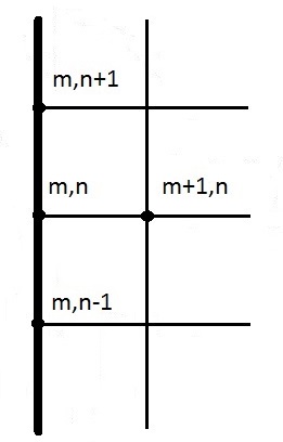
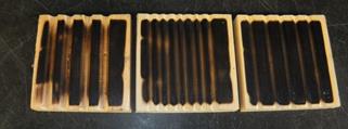
Photos were taken to document the difference in decomposition for case #3, 5, 7 and 11. Comparing the decomposition zone with the isosurface plot of the two-dimensional analysis, the appearance was found to fit very well. For case #3 a wave was observed - see Figure 16 - and for case #5 a straight line. For case #7 the appearance was less wavy than for case #3. For case #11 the decomposition zone and the temperature distribution were evenly into the sample.

Photos were taken of the upper surface and compared with the isosurface plots of case #6, #7 and #10. The greatest colour changes were for case #6 and the least for case #7 where unaffected parts could be found. The colour change of case #6 corresponds to the extensive temperature penetration of the three cases. The largely unaffected gauges of case #7 can be linked to the lower gauge temperatures. See Figure 17 and 18.

The similarities of the extension of the decomposition zones versus the temperature zones of the isosurface plots further strengthens the usefulness of the model.

4. 8. Assumptions and further work

Uniform emissivity was assumed for the finite parts. This may be valid for specimen with smaller depths, but with larger depths charring may have started in the upper parts of the gauges while the lower parts may still be unaffected, and emissivity will vary. The two-dimensional analysis could be refined accordingly.  

Invariant convection was assumed. Roughness will affect flow patterns and the convective heat transfer. Even though features were milled into the specimen and no structures were interfering with the flow, the invariant convection assumption will have to be investigated further.

Experiments should be performed with other heat fluxes and depths. Preferably lower heat fluxes and larger depths. Lower heat fluxes and larger depths will most likely increase the importance and influence of surface roughness and structures on the potential ignition.

5. Conclusions

It was found that in five out of thirteen experimental cases the average ignition time showed significant difference when compared to the flat surface case, but no clear pattern related to the gauge characteristics was detected.

Two out of thirteen experimental cases for the upper surface and the gauge temperature showed significant difference when compared to the flat surface case.  These cases showed no clear pattern related to the gauge characteristics. Comparing the upper surface and gauge temperatures for each case showed significant temperature difference in three out of thirteen cases, again no clear pattern was detected.

Verifying the two-dimensional analysis, the resulting outputs were found to be consistent with the definition of the boundary conditions and the virtual enclosures for the gauges.

When studying the analysis results at the time of ignition, six out of thirteen cases for the upper surface temperature showed significant difference. Five out of thirteen cases for the upper third gauge slope temperature showed significant difference, but no clear pattern was detected.  Comparing the upper surface and upper third gauge slope temperatures showed significant temperature difference in two out of thirteen cases.

When comparing the experimental results with the analysis results, only two cases showed significant temperature difference and coincided in both experiments and analysis. 

In both experiments and the two-dimensional analysis with normalized roughness features in the range 2% to 10% a majority of the temperatures were within the one standard deviation variation and did not show any significant difference compared with the flat case, except when comparing the gauge bottom temperatures and upper surface temperatures of the two-dimensional analysis where significant difference was found in all cases.

A number of experiments were also conducted with a heat flux of 50 kW m^-2, but resulted in virtually no differences in ignition time. This suggests that the importance of surface roughness will increase with decreasing heat flux, for example when the distance between the fire and the fuel item increases or when the heat release rate decreases. In a mine drift where the distance between different combustible components, equipment etc. can be substantial, the surface roughness and surface structures may influence the time to ignition as well as the likelihood of ignition.

Acknowledgement

Rickard Hansen conducted the work at Worcester Polytechnic Institute as part of his doctoral studies at Mälardalen University.

Randall Harris, Fire Laboratory Manager at Worcester Polytechnic Institute, is acknowledged for valuable assistance during the fire experiments.

References

[1] R. Hansen, “Analysis of Methodologies for Calculating the Heat Release Rates of Mining Vehicle Fires in Underground Mines,” Fire Safety Journal, vol. 71, pp. 194–216, 2015a.
[2] R. Hansen, “Study of Heat Release Rates of Mining Vehicles in Underground Hard Rock Mines,” Ph.D. dissertation, Mälardalen University, Västerås, 2015b.
[3] ‘Data book, off-the-road-tires’ (Off-The-Road Tire Department, Bridgestone Corporation, Tokyo), 2016
[4] R. Hansen, “Fire behavior of mining vehicles in underground hard rock mines,” International Journal of Mining Science and Technology, vol. 27, pp. 627-634, 2017.
[5] G. Heskestad, “Ease of ignition of fabrics exposed to flaming heat sources,” Journal of Consumer Product Flammability, vol. 6, pp. 28-88, 1979.
[6] K. Akita, “Studies on the Mechanism of Ignition of Wood,” Report of Fire Research Institute of Japan, vol. 9, pp. 1-44, 51-54, 77-83, 99-105, 1959.
[7] T. R. Thomas, Rough Surfaces. London: Imperial College Press, 1999.
[8] A. Atreya, “Ignition of fires,” Philosophical Transactions: Mathematical, Physical and Engineering Sciences, vol. 356, pp. 2787-2813, 1998.
[9] V. Babrauskas, Ignition Handbook. Issaquah: Fire Science Publishers, 2003.
[10] J. G. Quintiere, Fundamentals of fire phenomena. Hoboken: John Wiley & Sons Inc., 2006.
[11] J. P. Holman, Heat Transfer 9th edition. New York: McGraw-Hill, 2002.
[12] W. M. Lewandowski, E. Radziemska, M. Buzuk and H. Bieszk, “Free convection heat transfer and fluid flow above horizontal rectangular plates,” Applied Energy, vol. 66, pp. 177-197, 2000. View Article
[13] C. L. Tien, K. Y. Lee and A. J. Stretton, "Radiation Heat Transfer" in The SFPE Handbook of Fire Protection Engineering (P. J. DiNenno, D. Drysdale, C. L. Beyler, W. D. Walton, R. L. P. Custer, J. R. Hall, and J. M. Watts, Eds.), NFPA, Quincy, USA, 2008.
[14] M. T. Wilson, B. Z. Diugogorski and E. M. Kennedy EM, “Uniformity of Radiant Heat Fluxes in Cone Calorimeter,” Fire Safety Science, vol. 7, pp. 815-826, 2003.
[15] P. Schröder and P. Hanrahan P, “On the form factor between two polygons,” Computer Graphics, Proc., Ann. Conf. Series, SIGGRAPH 93, pp. 163-164, 1993.
[16] R. Siegel and J. R. Howell, Thermal Radiation Heat Transfer 4th edition. Washington: Taylor and Francis-Hemisphere, 2001.